Download the paper slide rule          Practice with the virtual slide rule

Slide rule tutorial

This is a brief tutorial to introduce the use of the slide rule.

A full and exaustive version can be also freely downloaded.

The mathematician John Napier discovered in 1614 the logarithms, published in "Mirifici logarithmorum canonis descriptio", capable of expressing any positive number via powers.
Since the product of two powers with the same base is a power with the same base and exponent given by the sum of the exponents, with logarithms multiplications and divisions can be made as simple additions and subtractions.

To multiply two numbers just look out for their logarithms and add them together: the result is the number whose logarithm correspond to the sum.
In practice the logarithm of a number in a certain base is the exponent to which the base must be raised to obtain the number.
The logarithm of 10,000 in base 10 is 4 (10⁴ = 10,000) and 10,000 x 1,000 become 10⁴x10³ = 10⁴⁺³ = 10⁷ = 10,000,000.
Multiplication and division of exponents allow to find squares, cubes and roots. Things get complicated when dealing numbers other than 10: we need a volume with more than a million values.
The tables had a very long life as they were cheap and their precision made them indispensable for astronomers and navigators ap to ca 1975.

With logarithms we are unable to work quickly as the consultation of the tables is very laborious.
In 1620 Edmund Gunter, to expedite the proceedings, designed the logarithmic scale by placing numbers on a ruler at a distance from the origin proportional to the value of their logarithm. Here is the table:

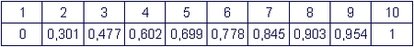
Now we can try to construct the scale: the 1 is the starting point, the 2 is located at 3.01 cm, the 3 to 4.77 and so on up to 10.
We can therefore represent each number as we can read, for example, the number 3 as 30, 300, 0.003, 0.3, etc.

How far it is possible, for reasons of space, we now add the minor divisions (logs between 1 and 99). Instead of search the logarithms in the tables we can simply add them with the help of a compass.
Calculating with a compass was however laborious, slow and difficult. In 1622 William Oughtred marked the logarithmic scales on two sliding parallel rulers. An innovation that allows the direct reading of the result.
The slide rule was born.

The sliderule, being an analog instrument, replace the mathematical functions with linear measurements. To show how it works let's start to see how we can execute an addition using two common metric rules.
To add 2 and 4, align first the 0 of the rule B with the 2 of the rule A.
We have set 2+ and the sum can be read on the mark of slide A, corresponding to the second addendum.

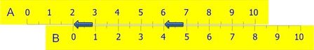
To add 2+6 we don't need to move again the rule (set on 2+), but just read the sum directly on the figure 6 of the B rule. To subtract, we use the opposite proceeding.

From the accuracy of the construction depends the precision of the results but, also dividing further the scales, it is not possible to operate with numbers greater than 100.
It 'is therefore clear that, as regards the addition and subtraction, the slide rule is much less practical than the abacus and to any other type of calculator. This system, however, becomes very powerful if the scales are drawn using the logarithmic succession that we have seen previously.

To perform 2 x 4 we align the 1 of scale B in correspondence of 2 in scale A and the result can be read on the same scale above the 4 of scale B.

We now have a tool that can perform multiplication. The previous picture also shows how to perform 8/4. Just put the 4 of scale B under the 8 of scale A and read the result on the same scale above the 1 in scale B.

There are also some disadvantages. If we want process 4x3 the slides are positioned as follows:

The total is now located out of the scale. To solve this problem, we need to use the 10 of the rule B, instead of the previous 1:

So we obtain 1.2, but the right total is 12: the slide rule gives only the numbers and how to locate the dot or how to add ten or hundreds we must find by ourselves.

Esempi pratici

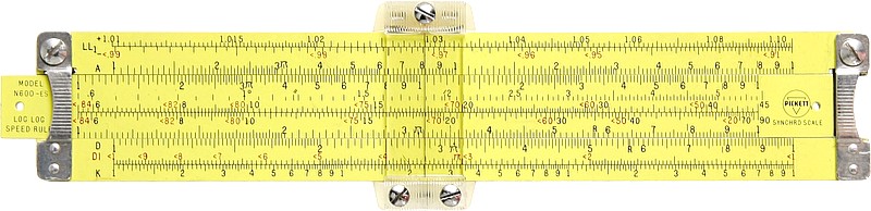
In the slide rules the scales are indicated by letters: the two most important are on the slide (C) and on the body (D). The others are used to simplify the calculations when you are in the presence of square roots (A and B), cubes and cube roots (K), exponential (LL), etc. up to more than 30.

Multiplication (uses C and D scales)

E.g. 2,3 x 3,4

• slide the C leftmost '1' on by side 2.3 on the D scale;
• move the cursor by side 3.4 on the C scale;
• the cursor is on the D scale just a bit over 7.8. The correct answer is 7.82.

Division (uses C and D scales)

E.g. 4,5 / 7,8

• move the cursor by side 4.5 on the D scale;
• slide 7.8 on the C scale by side the cursor;
• the C rightmost '1' is now at 5.76 on the D scale. We know that the result of 4/8 is near 0.5, so we adjust the decimal place to get 0.576. The correct answer is 0.576.

Squares and square roots (uses C and B scales)

E.g. square of 4,7

• move the cursor to 4.7 on the C scale;
• the cursor is now at 2.2 on the B scale;
• adjust by brain the decimal place: the correct answer is 22.

E.g. of a combined operation: √350 / 1,51

• the A and B scales have two similar halves. The left half is used to find the square root of numbers with odd numbers of digits; the right half is used for numbers with even numbers of digits. Since 350 has an even number of digits (3) we'll use the left half of the scale.
• moving the cursor by side the 350 of the A scale (odd number of digits, then the left side) we get its square root, 18.7, on the D scale;
• now we match 18.7 with 1.51 of the C scale: on the D scale, in correspondence with the C leftmost index '1', we can read the answer: ca. 12.35.

An electronic calculator would have been just a little more precise, finding 12.3896. This slight approxi-mation has not prevented von Braun to design space stations and send Man on the Moon. The slide rule is in fact less difficult than it sounds and the only secret is just to practice, for example with this virtual simulation.

Practice with this slide rule emulator

Links to other tutorials:

The Oughtred Society
The Slide Rule Museum

© 2004 - 2026 Nicola Marras Manfredi